S-Cube | Revolutionary Seismic Imaging with XWI Technology

Key takeaways

▹A complex Gulf of Mexico salt model was built entirely from scratch — no salt, no picked horizons, no well data — starting from a 1D compaction trend that was systematically wrong by up to 2500 m/s.
▹Highly dynamic parameterisations — changing constraints and misfit functions stage by stage — let the workflow self-correct both the salt and the sub-salt velocity trend.
▹A new objective function, TSL-AWI, interleaved with RWI, resolved a target layer in the low-illumination zone beneath the salt.
▹The result was validated against blind well logs and a quantitative trace-fit metric, outperforming conventional least-squares FWI despite starting from a worse model.

Subsalt imaging in the Gulf of Mexico is one of the hardest problems in applied geophysics. The high, heterogeneous velocity of salt bends ray-paths, scatters energy, and casts long illumination shadows over the very reservoirs explorers care about. Conventional velocity model building answers this with months of preprocessing, tomography, horizon picking, salt flooding, and iterative scenario testing — a labour-intensive process that leans heavily on human interpretation and, ultimately, on the accuracy of an initial model.

In our work at Alaminos Canyon, in partnership with Shell, we set out to answer a more demanding question: how far can Full-Waveform Inversion (FWI) be pushed if we hand it nothing to start from? No salt bodies. No picked horizons. No well data. Just raw field data and a starting model so simple it is systematically wrong almost everywhere.

The transformation at a glance

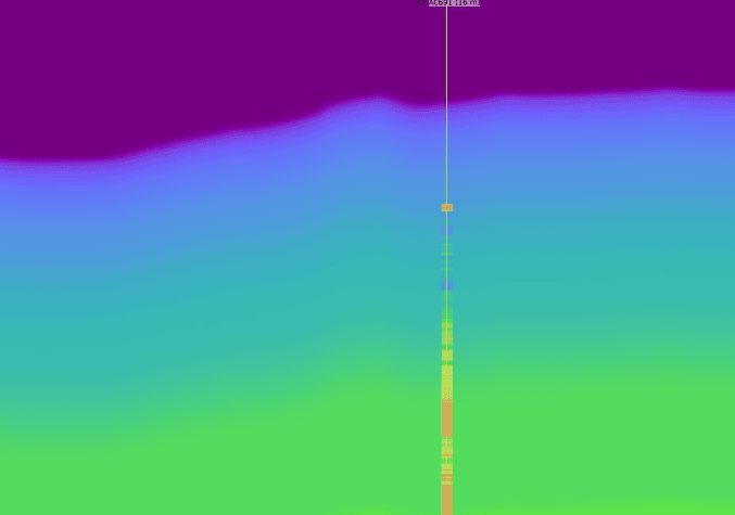
Before the detail, here is where we start and where we finish. On the left, a featureless 1D compaction trend with no salt. On the right, the final, blind-well-validated model. Everything in between was recovered by the data.

Final validated salt model — Drag to compare — The same cross-section, with the blind well overlaid: from a deliberately-wrong 1D start (left) to the final high-definition salt model (right).

Starting 1D compaction trend model — Drag to compare — The same cross-section, with the blind well overlaid: from a deliberately-wrong 1D start (left) to the final high-definition salt model (right).

The dataset: Alaminos Canyon

The study uses unprocessed hydrophone-only records from a modern ocean-bottom node (OBN) acquisition in the Gulf of Mexico, covering roughly 600 km² in water depths close to 2 km. Nodes sit on a 400 m × 400 m grid, with shots every 50 m inline and crossline from a conventional airgun source. While the geometry allows offsets approaching 30 km, that maximum is available only for a handful of midpoints near the survey centre — for most azimuths and midpoints, usable offsets are at or below 20 km. In other words, no exceptionally long offsets and no unusually low frequencies to lean on.

Starting from a model that is wrong on purpose

The workflow begins with a one-dimensional sedimentary compaction trend that was suspected to be systematically in error, with local velocity errors in excess of 1500 m/s — rising to 2500 m/s where salt is present. The model is isotropic, containing only an accurate seabed and water column; there is no salt in it at all. For the lowest frequencies in the field data, this start model is cycle-skipped almost everywhere, often by several cycles. Conventional least-squares FWI cannot recover from this. The self-correcting scheme is designed precisely so that it can.

Step 0: 1D compaction trend starting model — Step 0 — The starting point: a near one-dimensional compaction trend. No salt, isotropic, and systematically in error by up to 2500 m/s.

Self-correction through dynamic parameterisation

The engine underneath every stage is Adaptive Waveform Inversion (AWI) — a family of FWI objective functions whose misfit surfaces do not contain the local minima responsible for cycle skipping. Rather than comparing traces sample by sample, AWI derives matching filters that map observed data onto predicted data, and drives those filters towards zero-lag delta functions. What makes the salt model emerge is not a single algorithm but a sequence of them: the parameterisation, constraints, and misfit formulation change dynamically as the model evolves.

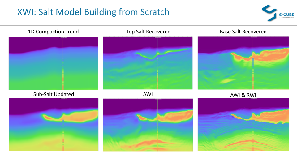
Early iterations use an accelerated, more-aggressive misfit function together with simple constraints, taking large steps to push background velocities in the right direction and to build a smooth salt body with the correct long-wavelength geometry. Unconstrained AWI first captures the top of salt as a thin high-velocity layer.

Step 1: Unconstrained AWI captures top salt — Step 1 — Unconstrained AWI builds a thin high-velocity layer marking the top of the salt body, and begins broadly-correct shallow sedimentary corrections.

Constrained AWI (cAWI) then imposes two constraints: that the model stay smooth, and that velocity not decrease with depth. The second behaves like salt flooding — but crucially it requires no top-salt pick and no assumed flood velocity. The data itself demands high velocities at the top of salt, and the constraint only lets those velocities appear if they extend to the base of the model.

Step 2: Constrained AWI floods the model — Step 2 — Constrained AWI (cAWI) effectively floods the model with salt velocity — without picking a top-salt horizon or specifying a flood velocity.

Relaxing those constraints lets the model roughen and velocities begin to fall where the base of salt will later appear.

Step 3: Relaxing the constraints on AWI — Step 3 — As the flooding constraint is relaxed, the model roughens and velocity starts to reduce at the position where base salt will subsequently emerge.

A second constraint then pulls the model back towards the original compaction trend wherever doing so does not significantly worsen the fit to the data — algorithmically, both a constraint on the model and a penalty on the data. The result is a smooth salt body superimposed on a smooth sedimentary trend.

Step 4: Apply a new constraint on AWI — Step 4 — A new constraint restores the sedimentary compaction trend below a smooth base of salt wherever the data permit, leaving a clean salt body on a coherent background.

Step 5: Relaxing the constraints on AWI again — Step 5 — Constraints are relaxed again, allowing the inversion to add detail now that the macro-scale salt geometry is broadly correct.

Correcting the sub-salt trend

This is where the self-correcting loop earns its name. Part-way through the workflow, the spatial variation of several independent data-misfit measures is used to reveal where the assumed sedimentary trend was wrong. The phase misfit for turning rays and wide-angle reflections indicates the smooth corrections the trend needs, and VTI anisotropy is introduced at this stage. The sub-salt trend is updated — a large, approximate adjustment in keeping with the accelerated strategy — and further passes of AWI using both refracted and reflected energy (rAWI) build sub-salt structure.

Step 6: Sub-salt trend updated — Step 6 — Independent misfit measures localise where the sedimentary trend was in error; the sub-salt velocity trend is corrected and anisotropy is introduced.

Step 7: AWI continues subsalt — Step 7 — Reflection-inclusive AWI (rAWI) continues to build sub-salt structure now that the background trend beneath the salt is on the right footing.

The accelerated formulation is fast and cheap, but it can overshoot, leaving localised artefacts. A final, more-benign AWI formulation is unable to make large macro-scale changes but excels at the fine detail — removing spurious structure and repairing regions where earlier corrections went too far.

Step 8: Fine-tuned AWI — Step 8 — A less-aggressive AWI formulation removes the artefacts left by the accelerated stages and sharpens spatial resolution, leaving an accurate, artefact-free model.

TSL-AWI and the interplay with RWI

The most recent step forward is a new objective function we call Time-Space-Lag Adaptive Waveform Inversion (TSL-AWI). Where standard AWI uses single-trace matching filters, TSL-AWI uses multi-dimensional filters — multi-trace deconvolution — so it captures both temporal and spatial residual moveout and is sensitive to both reflection and refraction errors. That gives it faster, more global convergence from a poor start.

Interleaving TSL-AWI with Reflection Waveform Inversion (RWI) on the raw data proved decisive in the hardest areas: macro-level correction of the salt and sub-salt velocity trends, building sub-salt reflectivity, and sharpening general salt definition. Together these functionals take the model from a poor compaction trend to a final result in a fraction of the elapsed time — and cost — of a conventional model-building cycle.

Step 9: AWI-RWI — Step 9 — Interleaved TSL-AWI / RWI on raw field data delivers the macro-level corrections to salt and sub-salt trends that are hardest to achieve from a poor starting model.

From velocity to image

With an accurate acoustic velocity model in hand, a single impedance inversion (iAWI) pass — updating for acoustic impedance assuming no change in velocity, inverting over a restricted offset range to mitigate elastic effects, with long wavelengths removed via a Laplacian filter — produces a low-cost, bandlimited, RTM-like reflectivity image directly from unprocessed field data. This doubles as a rapid QC throughout the workflow.

Step 10: Impedance Inversion — Step 10 — Impedance inversion (iAWI) generates a bandlimited reflectivity image straight from the raw data — a fast, standalone QC of the evolving model.

RTM at 15Hz — Imaging — Reverse-time migration at 15 Hz on the final model. The velocity model is accurate and well resolved enough to image cleanly beneath the salt.

FWI-derived reflectivity at 8Hz — Imaging — FWI-derived reflectivity at 8 Hz. Even at low frequency, the structurally simple sub-salt reflectivity confirms the model's accuracy in the low-illumination target zone.

Validation against blind wells

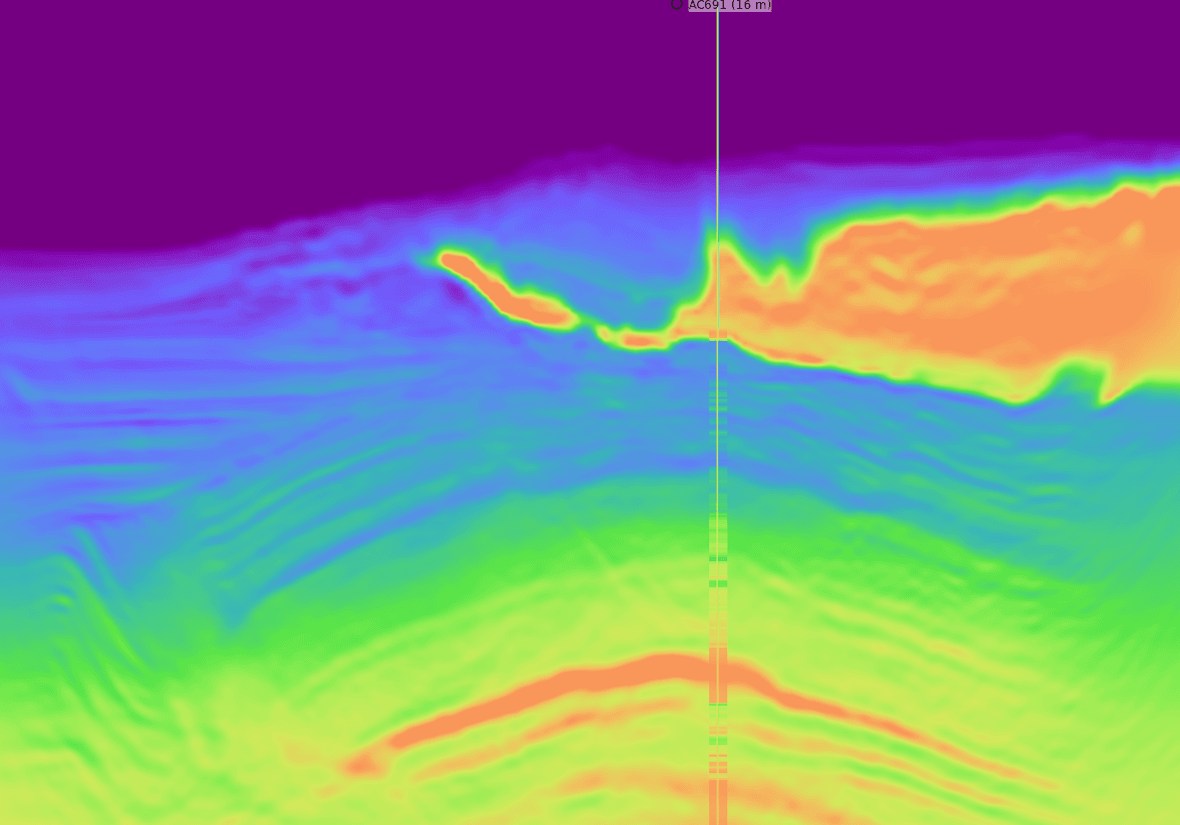
A model built without any well input is only as convincing as its validation. The step-by-step improvement is tracked against a blind well log that played no part in the inversion — it was withheld until the very end of the project. Compared against that blind log, TSL-AWI more accurately recovers the top and base of salt, the deeper high-velocity layers, and the low-velocity target reservoir than conventional least-squares FWI — even though it began from a worse model, with a simpler salt geometry and no knowledge of the high-velocity layers beneath the salt.

The accuracy is confirmed quantitatively too. A trace-fit metric — seismic data correlation mapped across the survey and projected along each inline — shows the TSL-AWI model delivering the best data fit of three model generations: the clearest possible sign that the recovered velocities are real, not artefacts of a favourable starting point.

Final salt model results validated against blind wells — Result — The final salt model. Validated against blind well logs and a quantitative trace-fit metric, TSL-AWI + RWI outperforms conventional FWI despite starting from a less accurate model.

Why this matters

The conventional route to a salt-ready velocity model — processing, tomography, horizon picking, scenario testing, repeated manual intervention — is expensive, slow, and dependent on interpretation choices made early and rarely revisited. What Alaminos Canyon demonstrates is that a data-driven, automated, self-correcting workflow can start from a model whose only real features are the seabed and water column and still arrive at a high-definition, blind-well-validated result — fit for immediate high-frequency multi-parameter elastic FWI.

The economics follow from the design. The accelerated early stages take large steps with minimal compute, and the entire sequence is automated and pre-defined — high-level, QC-driven decisions steer the model around the central self-correcting loop, with no manual picking or scenario testing in between. And where a legacy velocity model already exists, heavily smoothing it produces a starting point equivalent to the mid-sequence model: the workflow can pick up from there, circumventing the earlier constrained stages entirely.

For exploration teams, that means less time and cost to first image, fewer subjective decisions baked into the model, and a defensible, quantitative chain of evidence for the target layer sitting in salt's shadow. The interplay of TSL-AWI and RWI turns the hardest starting conditions into a solved problem — and pushes acoustic salt-model building close to the physical limits of the modelling kernel.

Have a salt problem of your own?

If your subsalt targets sit in shadow — or your legacy velocity model is holding your imaging back — we would like to hear about it. Let's talk about what XWI can recover from your data.

Talk to our team

Explore further

Based on work presented at IMAGE 2026, Houston, as “Breaking Through Complex Salt: Harnessing the Interplay of Time-Space-Lag Adaptive Waveform Inversion and Reflection Waveform Inversion” (N. Shah, A. Kovacs, C. Mavropoulos, T. Oxford — S-Cube; M. Liu — Shell). The authors thank Shell for permission to present this work and to use the dataset shown.

Breaking Through Complex Salt: Building a Gulf of Mexico Salt Model From Scratch